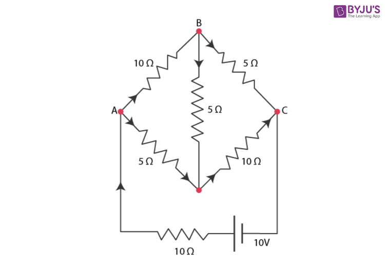
The current flowing through various branches of the network is shown in the figure given below:

Let I 1 be the current flowing through the outer circuit
Let I 2 be the current flowing through AB branch
Let I 3 be the current flowing through AD branch
Let I 2 – I 4 be the current flowing through branch BC
Let I 3 + I 4 be the current flowing through branch DC
Let us take closed-circuit ABDA into consideration, we know that potential is zero.
i.e , 10 I 2 + 5 I 4 – 5 I 3 = 0
2 I 2 + I 4 – I 3 = 0
I 3 = 2 I 2 + I 4 . . . . . . . . . . . . . . . . . . . . . . eq ( 1 )
Let us take closed circuit BCDB into consideration, we know that potential is zero.
i.e., 5 ( I 2 – I 4 ) – 10 ( I 3 + I 4 ) – 5 I 4 = 0
5 I 2 – 5 I 4 – 10 I 3 – 10 I 4 – 5 I 4 = 0
5 I 2 – 10 I 3 – 20 I 4 = 0
I 2 = 2 I 3 – 4 I 4 . . . . . . . . . . . . . . . . . . . . . . eq ( 2 )
Let us take closed-circuit ABCFEA into consideration, we know that potential is zero.
i.e , – 10 + 10 ( I 1 ) + 10 ( I 2 ) + 5 ( I 2 – I 4 ) = 0
10 = 15 I 2 + 10 I 1 – 5 I 4
3 I 2 + 2 I 2 – I 4 = 2 . . . . . . . . . . . . . . . . . . . . . . eq ( 3 )
From equation ( 1 ) and ( 2 ), we have :
I 3 = 2 ( 2 I 3 + 4 I 4 ) + I 4
I 3 = 4 I 3 + 8 I 4 + I 4
– 3 I 3 = 9 I 4
– 3 I 4 = + I 3 . . . . . . . . . . . . . . . . . . . . . . eq ( 4 )
Putting equation ( 4 ) in equation ( 1 ) , we have :
I 3 = 2 I 2 + I 4
– 4 I 4 = 2 I 2
I 2 = – 2 I 4 . . . . . . . . . . . . . . . . . . . . . . eq ( 5 )
From the above equation , we infer that :
I 1 = I 3 + I 2 . . . . . . . . . . . . . . . . . . . . . . eq ( 6 )
Putting equation ( 4 ) in equation ( 1 ), we obtain
3 I 2 + 2 ( I 3 + I 2 ) – I 4 = 2
5 I 2 + 2 I 3 – I 4 = 2 . . . . . . . . . . . . . . . . . . . . . . eq ( 7 )
Putting equations ( 4 ) and ( 5 ) in equation ( 7 ), we obtain
5 ( – 2 I 4 ) + 2 ( – 3 I 4 ) – I 4 = 2
– 10 I 4 – 6 I 4 – I 4 = 2
17 I 4 = – 2
\(\begin{array}{l}I _{ 4 } = \frac{ – 2 }{ 17 } A\end{array} \)
Equation ( 4 ) reduces to
I 3 = – 3 ( I 4 )
\(\begin{array}{l}I_{ 3 } = – 3 \left ( \frac{ – 2 }{ 17 } \right ) = \frac{ 6 }{ 17 } A\end{array} \)
I 2 = – 2 ( I 4 )
\(\begin{array}{l}I_{ 2 } = – 2 \left ( \frac{ – 2 }{ 17 } \right ) = \frac{ 4 }{ 17 } A\end{array} \)
\(\begin{array}{l}I _{ 2 } – I _{ 4 } = \frac{ 4 }{ 17 } – \frac{ – 2 }{ 17 } = \frac{ 6 }{ 17 } A\end{array} \)
\(\begin{array}{l}I _{ 3 } + I _{ 4 } = \frac{ 6 }{ 17 } – \frac{ – 2 }{ 17 } = \frac{ 4 }{ 17 } A\end{array} \)
\(\begin{array}{l}I _{ 1 } = I _{ 3 } + I _{ 2 }\end{array} \)
\(\begin{array}{l}I _{ 1 } = \frac{ 6 }{ 17 } + \frac{ 4 }{ 17 } = \frac{ 10 }{ 17 } A\end{array} \)
Therefore, current in each branch is given as :
In branch
\(\begin{array}{l}AB = \frac{ 4 }{ 17 } A\end{array} \)
In branch
\(\begin{array}{l}BC = \frac{ 6 }{ 17 } A\end{array} \)
In branch
\(\begin{array}{l}CD = \frac{ – 4 }{ 17 } A\end{array} \)
In branch
\(\begin{array}{l}AD = \frac{ 6 }{ 17 } A\end{array} \)
In branch
\(\begin{array}{l}BD = \frac{ – 2 }{ 17 } A\end{array} \)
Total current
\(\begin{array}{l}= \frac{ 4 }{ 17 } + \frac{ 6 }{ 17 } + \frac{ – 4 }{ 17 } + \frac{ 6 }{ 17 } + \frac{ – 2 }{ 17 } = \frac{ 10 }{ 17 } A\end{array} \)