Interpolation and Numerical Integration - Numerical Methods - Engineering Sciences Previous Year Questions

1

2007 · Engineering Sciences · Numerical Methods · Interpolation and Numerical Integration

Engineering Sciences (XE) 2007

If a polynomial of degree three interpolates a function $f(x)$ at the points $(0, 3)$, $(1, 13), (3, 99)$ and $(4, 187)$, then $f(2)$ is

A

20

B

36

C

43

D

58

Open complete paper

2

2007 · Engineering Sciences · Numerical Methods · Interpolation and Numerical Integration

Engineering Sciences (XE) 2007

If \( y_i \) denotes the value of y(x) at \( x = x_i \) in \( x_0 < x_1 < ... < x_i < ... < x_n \) and \( x_i - x_{i-1} = h \) for \( 1 \leq i \leq n \), then \( \frac{d^2 y}{dx^2} \) at \( x = x_i \), \( 1 \leq i \leq n-1 \) is approximated using finite difference scheme by

A

\(\frac{1}{2h} ( y_{i+1} - 2y_i + y_{i-1} )\)

B

\(\frac{1}{2h} ( y_{i+1} - y_i + y_{i-1} )\)

C

\(\frac{1}{h^2} ( y_{i+1} - 2y_i + y_{i-1} )\)

D

\(\frac{1}{h^2} ( y_{i+1} - y_i + y_{i-1} )\)

Open complete paper

3

2007 · Engineering Sciences · Numerical Methods · Interpolation and Numerical Integration

Engineering Sciences (XE) 2007

The graph of a function \( y = f(x) \) passes through the points (0, -3), (1, -1) and (2, 3). Using Lagrange interpolation, the value of x at which the curve crosses the x-axis is obtained as

A

1.375

B

1.475

C

1.575

D

1.675

Open complete paper

4

2007 · Engineering Sciences · Numerical Methods · Interpolation and Numerical Integration

Engineering Sciences (XE) 2007

The area bounded by the curve \(y = 1 - x^2\) and the x-axis from \(x = -1\) to \(x = 1\) using Trapezoidal rule with step length \(h = 0.5\) is

A

1.20

B

1.23

C

1.25

D

1.33

Open complete paper

5

2007 · Engineering Sciences · Numerical Methods · Interpolation and Numerical Integration

Engineering Sciences (XE) 2007

If the above formula is used as Simpson’s 1/3 rule, then

A

b = d = 1

B

b = d = 2

C

b = 2d = 1

D

b = 2d = 2

Open complete paper

6

2007 · Engineering Sciences · Numerical Methods · Interpolation and Numerical Integration

Engineering Sciences (XE) 2007

Using the correct values of b and d from Q.25 in the quadrature formula the value of \(\int_{0}^{1} \frac{12}{1+x} dx\) evaluated correct up to 4 decimal places is

A

8.3091

B

8.3121

C

8.3151

D

8.3191

Open complete paper

7

2008 · Engineering Sciences · Numerical Methods · Interpolation and Numerical Integration

Engineering Sciences (XE) 2008

Evaluation of the integral \[\int_{0}^{1} \frac{dx}{\sqrt{1+x^2}}\] using 2 segment trapezoidal rule with equal intervals gives the result

A

0.566

B

0.564

C

0.562

D

0.560

Open complete paper

8

2008 · Engineering Sciences · Numerical Methods · Interpolation and Numerical Integration

Engineering Sciences (XE) 2008

The value of the integral \[\int_{1}^{2} \frac{dx}{x}\] obtained by using Simpson's 1/3 rule, with 3 points, is

A

0.694

B

0.693

C

0.692

D

0.691

Open complete paper

9

2008 · Engineering Sciences · Numerical Methods · Interpolation and Numerical Integration

Engineering Sciences (XE) 2008

A quadrature formula is given by \[ \int_{0}^{1} f(x)dx = pf(0) + qf(0.5) + rf(1) \] where the coefficients \( p, q, \) and \( r \) are determined by comparing the right hand side of the above formula with the exact value of the integral for a quadratic polynomial. The formula corresponds to

A

Two segment trapezoidal rule

B

One segment trapezoidal rule

C

Simpson’s 3/8 rule

D

Simpson’s 1/3 rule

Open complete paper

10

2008 · Engineering Sciences · Numerical Methods · Interpolation and Numerical Integration

Engineering Sciences (XE) 2008

For a function \( f(x) \) whose second derivative \( f''(x) \) has a maximum value 12 in the interval [0,1]. The number of segments required to integrate \( \int_{0}^{1} f(x)dx \) with an accuracy of 0.0001 using trapezoidal rule is

A

10

B

12

C

100

D

1000

Open complete paper

11

2008 · Engineering Sciences · Numerical Methods · Interpolation and Numerical Integration

Engineering Sciences (XE) 2008

The value of f'(x) at x = 0.5 accurate upto two decimal places, is

A

0.82

B

0.85

C

0.88

D

0.91

Open complete paper

12

2008 · Engineering Sciences · Numerical Methods · Interpolation and Numerical Integration

Engineering Sciences (XE) 2008

The value of f'(x) at x = 0.55 obtained using Newton's interpolation formula, is

A

0.5626

B

0.5227

C

0.4847

D

0.4749

Open complete paper

13

2008 · Engineering Sciences · Numerical Methods · Interpolation and Numerical Integration

Engineering Sciences (XE) 2008

The function may be represented by a polynomial $P(x)=(x-a)R(x)$, where $R(x)$ is a polynomial of degree 2, obtained by Lagrange’s interpolation and $a$ is a real constant. The polynomial $R(x)$ is

A

$x^2 + 6x + 12$

B

$x^2 + 6x -12$

C

$x^2 - 6x -12$

D

$x^2 - 6x + 12$

Open complete paper

14

2008 · Engineering Sciences · Numerical Methods · Interpolation and Numerical Integration

Engineering Sciences (XE) 2008

The value of the derivative of the interpolated polynomial $P(x)$ at the position of its real root is

A

$-6$

B

$-4$

C

$6$

D

$7$

Open complete paper

15

2009 · Engineering Sciences · Numerical Methods · Interpolation and Numerical Integration

Engineering Sciences (XE) 2009

Simpson’s 1/3 rule applied to \(\int_{-1}^{1}(3x^{2}+5)dx\), with sub-interval \(h =1\), will give

A

the exact result

B

error between 0.01% to 0.1%

C

error between 0.1% to 1.0%

D

error > 1.0 %

Open complete paper

16

2010 · Engineering Sciences · Numerical Methods · Interpolation and Numerical Integration

Engineering Sciences (XE) 2010

If the quadrature rule \( \int_{0}^{3} f(x) dx = \alpha f(1) + \beta f(3) \) is exact for all polynomials of degree 2 or less, then

A

\(\alpha = 3/4, \beta = 3/4 \)

B

\(\alpha = 3/4, \beta = 9/4 \)

C

\(\alpha = 9/4, \beta = 3/4 \)

D

\(\alpha = 9/4, \beta = 9/4 \)

Open complete paper

17

2011 · Engineering Sciences · Numerical Methods · Interpolation and Numerical Integration

Engineering Sciences (XE) 2011

The fuel consumed by a motorcycle during a journey while traveling at various speeds is indicated in the graph below.

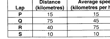
The distances covered during four laps of the journey are listed in the table below.

Lap	Distance (kilometres)	Average speed (kilometres per hour)
P	15	15
Q	75	45
R	40	75
S	10	10

From the given data, we can conclude that the fuel consumed per kilometre was least during the lap

A

P

B

Q

C

R

D

S

Open complete paper

18

2012 · Engineering Sciences · Numerical Methods · Interpolation and Numerical Integration

Engineering Sciences (XE) 2012

The exact solution of the integral \(\int_0^4 (x^2 - 4) dx\) is denoted by \(I_E\). The same integral evaluated numerically by the trapezoidal rule and the Simpson's 1/3 rule are denoted by \(I_T\) and \(I_S\), respectively. The subinterval used in the numerical methods is \(h = 2\). Then

A

\(I_E = I_S > I_T\)

B

\(I_E = I_S < I_T\)

C

\(I_E < I_S < I_T\)

D

\(I_E > I_S > I_T\)

Open complete paper

19

2016 · Engineering Sciences · Numerical Methods · Interpolation and Numerical Integration

Engineering Sciences (XE) 2016

Let \(P(x)\) and \(Q(x)\) be the polynomials of degree 5, generated by Lagrange and Newton interpolation methods respectively, both passing through given six distinct points on the xy-plane. Which of the following is correct?

A

\(P(x) \equiv Q(x)\)

B

\(P(x) - Q(x)\) is a polynomial of degree 1

C

\(P(x) - Q(x)\) is a polynomial of degree 2

D

\(P(x) - Q(x)\) is a polynomial of degree 3

Open complete paper

20

2017 · Engineering Sciences · Numerical Methods · Interpolation and Numerical Integration

Engineering Sciences (XE) 2017

Suppose \( \alpha, \beta, \gamma \) and \( \delta \) are constants such that \[ p(x) = \delta + \gamma (x+1) + \beta x(x+1) + \alpha x(x+1)(x-1) \] is the interpolating polynomial for the data \((-1, -3), (0,1), (1,-1), \) and \( (2, -3) \). Then the value of \( \gamma - \beta \) is ______________.

Check answer

Open complete paper